
TL;DR: Latency-tolerant architectures, e.g., GPUs, increasingly use memory/storage hierarchies, e.g., for KV Caches to speed Large-Language Model AI inference. To aid codesign of such workloads and architectures, we develop the simple PipeOrgan analytic model for bandwidth-bound workloads running on memory/storage hierarchies.
Background
For three reasons, memory bandwidth, more than latency, limits AI inference performance. First, AI inference uses latency-tolerant compute engines, such as GPUs. Second, it principally uses hardware memory hierarchies to store a data structure called a Key-Value (KV) Cache that holds information from recent queries to reduce redundant computation. With PagedAttention, each KV Cache fetch obtains one or more multi-megabyte blocks (often called pages) that require substantial bandwidth to complete. Third, inference’s “decode” phase is memory-bound due to low arithmetic intensity, putting great pressure on memory bandwidth.
Traditional CPU memory/storage hierarchies are shaped by increasing latency, but designing hierarchies for AI workloads requires focusing on decreasing bandwidth. Since AI software is flexible, codesigning software and hardware is essential.
To provide intuition and first answer to the above questions, we next contribute the simple PipeOrgan analytic model for optimizing bandwidth-bound workloads running on a memory hierarchy with many parallel pipes from memories to compute. The PipeOrgan model shows that husbanding and providing bandwidth is important for AI software and hardware. Analytic models have long provided computing intuition, e.g., Amdahl’s Law, Iron Law, and Roofline.
Example System with Two Parallel Memories
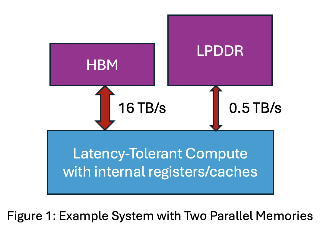
Let’s start simple. Consider the hardware depicted in Figure 1 with High Bandwidth Memory (HBM) with bandwidth 16 TB/s in parallel with an LPDDR memory with bandwidth 0.5 TB/s. Assume for now that there are no transfers between memories, e.g., to cache.
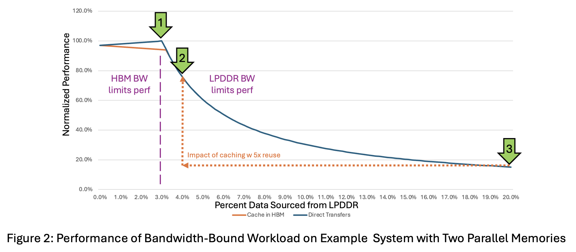
Using the PipeOrgan math from the next section, Figure 2’s blue line shows how system performance changes depending on what percentage of data comes from LPDDR memory. (The orange line comes later when we add caching.) Performance is highest when LPDDR provides exactly 3% of the data (arrow 1), which matches its 3% bandwidth (0.5/(16.0+0.5)). At this point, both LPDDR and HBM memories finish transferring data at the same time, so they act as co-bottlenecks and the system runs at peak efficiency.
When less than 3% of data is from LPDDR (left of the peak), HBM finishes last and limits performance. When LPDDR sources more than 3% (right of the peak), it is the bottleneck. LPDDR might have to source more data, because HBM’s limited capacity, currently 48-64GB per stack, may preclude it from being able to source its share (97%). If so, performance drops quickly: 4% from LPDDR gives 76% of peak (arrow 2), and 20% yields just 15% (arrow 3).
However, future AI systems will feature multiple memory and storage levels, using HBM, LPDDR, host DDR, pooled DDR, and attached or pooled FLASH storage.
PipeOrgan Model of Systems with N Parallel Memories
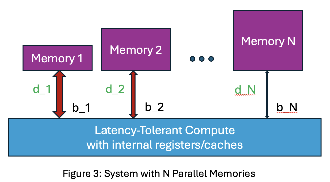
The above result generalizes to an N-level memory/storage hierarchy with each level feeding compute in parallel. Optimal performance is achieved when all parallel memories complete a workload phase simultaneously, leading to this PipeOrgan principle:
Memory-bandwidth-bound workloads perform best when data is sourced from each memory level in proportion to its bandwidth.
Proof:
- Let each memory provide bandwidth b_i TB/s in parallel for total bandwidth B = b_1 + … + b_N.
- For a workload, let each source d_i bytes in parallel for total data transferred D = d_1 + … + d_N.
- By assumption, the workload is limited by data transfer time with compute hidden.
- Time for each memory to finish its data transfer is d_i/b_i = TB/(TB/s) = seconds.
- Workload Time is the maximum of all memories finishing: MAX [d_1/b_1, …, d_N/b_N].
- Workload Performance = 1/ Time = MIN[b_1/d_1, …, b_N/d_N].
- Set each d_i = (D/B)*b_i = proportional to its bandwidth b_i.
- Performance = MIN[b_1/((D/B)*b_1), …, b_N/((D/B)*b_N)].
- Performance = MIN[(B/D), …, (B/D)] = B/D and Time = 1/Performance = D/B.
This makes sense: PipeOrgan shows that best performance occurs when one moves all the data using all the bandwidth with no bandwidth idling.
But Caching Is Critical
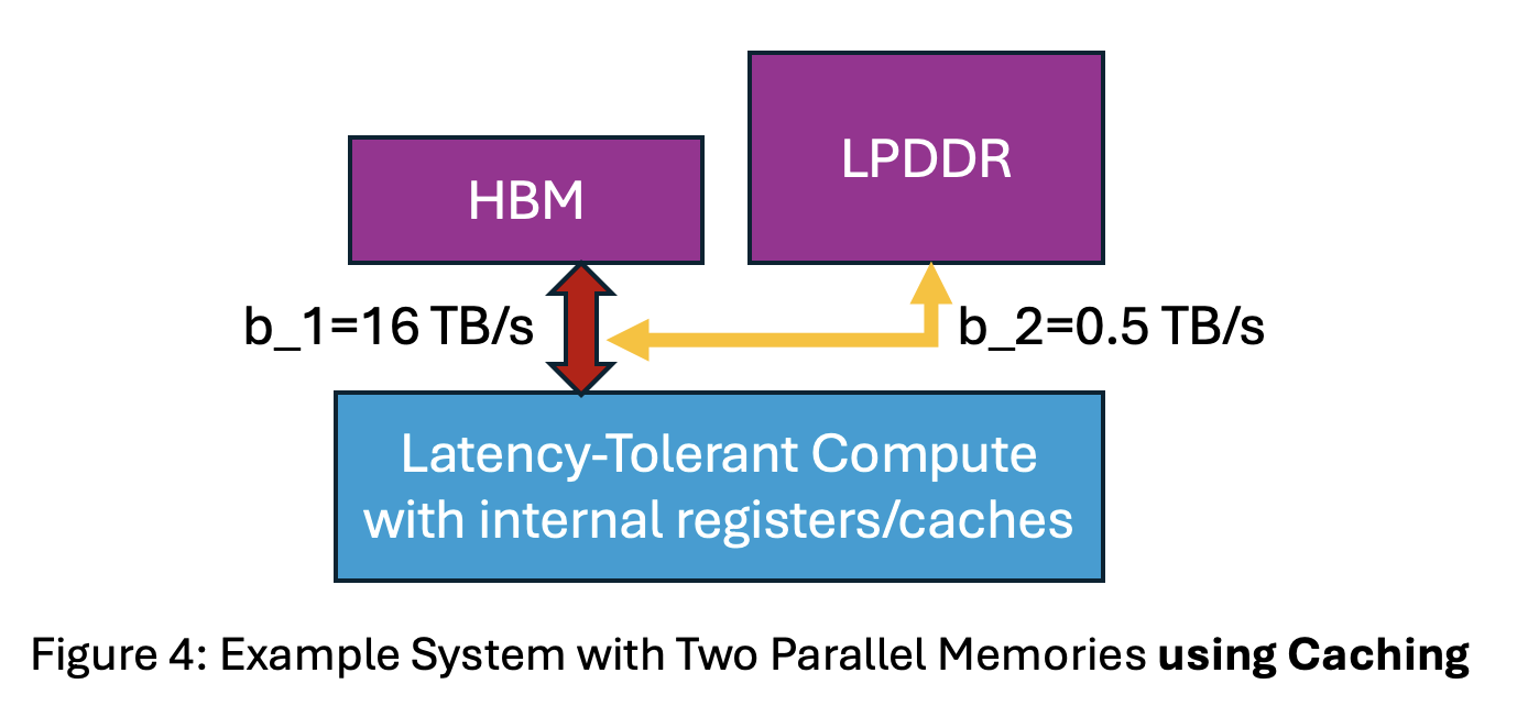
The PipeOrgan version above assumes all data goes directly to compute, without transfers among memories. In reality, systems move data from lower- to higher-bandwidth memories, caching it for reuse. For a two-level system (see Figure 4), assume the entire fraction of the workload’s data used from LPDDR is first transferred to HBM for caching (orange arrow). Let the data used from LPDDR be f*D where f ranges from 0 to 1.
- Performance with caching = MIN[(b_1/D)/(f+1), b_2/(f*D)] = MIN[limited by HBM BW, limited by LPDDR BW].
Figure 2 shows an orange curve for caching that is hidden under the original blue curve when more than 3% of data is sourced from LPDDR. At more than 3% from LPDDR, performance–without and with caching–is limited by the time to transfer needed data with the same limited LPDDR bandwidth.
While it might look like caching doesn’t matter, caching is actually important. This is because caching can greatly shift a workload’s x-axis operating point. For example, sourcing 20% of data from LPDDR yields 15% of peak performance (arrow 3). If LPDDR data is cached in HBM and reused five times, then–as the orange dashed arrow shows–only 4% comes from LPDDR and performance gets boosted to 76% of peak—a ~5x improvement (arrow 2).
Consequently, caching remains critical. Moreover, PipeOrgan and its N parallel memory principle also applies bandwidth-bound workloads once caching’s more complex information flows are accounted for.
Implications, Limitations and Future Work
Statistician George Box famously said, “Essentially, all models are wrong, but some are useful.”
We conjecture that the PipeOrgan model is useful for AI codesign, especially in the early stages and with software people having less hardware understanding. Its key implication is that bandwidth-bound workloads must carefully manage bandwidth from larger, slower memories and storage. While vast data can be stored statically, dynamic use from low-bandwidth memories should remain modest.
Three PipeOrgan limitations motivate future work. First, most workloads aren’t bandwidth bound throughout, and PipeOrgan doesn’t address other phases. Modeling these requires more parameters, increasing accuracy but also complexity.
Second, the caching model variant only covers two memory levels and always transfers data first to the higher-bandwidth level before use. Future work should extend this to N memory levels and more advanced caching policies. Modeling the many options for caching may be challenging.
Third, PipeOrgan may need to be extended for systems that do some processing in or near the memories themselves rather than moving all data to a segregated compute unit.
Burks, Goldstine, & von Neumann, 1946: We are therefore forced to recognize the possibility of constructing a hierarchy of memories, each of which has greater capacity than the preceding but which is less quickly accessible.
In sum, after eight decades of memory hierarchies focused mostly on latency, we are now at the exciting early stages of codesigning bandwidth-focused memory/storage hierarchies for more flexible AI software.
About the Author: Mark D. Hill is John P. Morgridge Professor and Gene M. Amdahl Professor Emeritus of Computer Sciences at the University of Wisconsin-Madison and consultant to industry. He initiated the PipeOrgan model consulting for Microsoft and was given permission to release it. He is a fellow of AAAS, ACM, and IEEE, as well as recipient of the 2019 Eckert-Mauchly Award.
Disclaimer: These posts are written by individual contributors to share their thoughts on the Computer Architecture Today blog for the benefit of the community. Any views or opinions represented in this blog are personal, belong solely to the blog author and do not represent those of ACM SIGARCH or its parent organization, ACM.