The Return of Rigorous Full-System Timing Simulation

Accurate timing simulation remains one of the most important tools in computer architecture, but modern systems have made cycle-level simulation increasingly impractical. Today’s platforms combine many-core CPUs, deep memory hierarchies, accelerators, complex I/O, and large software stacks, making detailed simulation extremely slow—often requiring months to simulate seconds of execution. This “timing simulation wall” has pushed researchers toward approximations such as application-only simulation, fixed instruction windows, or instruction windows representing only the workload. While these reduce runtime, they often sacrifice rigorous end-to-end measurement of real microarchitectural behavior.

This blog argues for a return to rigorous full-system timing simulation—not by simulating everything in detail at all times, but by measuring the right execution intervals, using the right performance metrics, and applying statistically sound methods to make accurate simulation practical again.

Why Full-System Simulation?

Full-system simulation emulates an entire computer system: CPU, memory, devices, operating system, and applications. Unlike user-level simulation, it captures interactions across the full software and hardware stack. Full-system simulation matters because many critical behaviors emerge from OS activity, interrupts, I/O, memory management, synchronization, and device interactions—not from application code alone. Ignoring these layers can misrepresent real system bottlenecks and performance.

Full-system simulation dates back to the 1990s with systems like SimOS, later influencing platforms such as Simics (now Intel Simics Simulator), M5 (integrated into gem5) and QEMU (used in MARSS and QFlex).

Today, full-system simulation is becoming essential again for four reasons:

1. Modern workloads are service-oriented and multi-tenant, relying on microservices, RPCs, storage stacks, and OS-mediated interactions.
2. Many server and mobile workloads spend significant time in the OS, making kernel behavior central to performance analysis.
3. Heterogeneous systems increasingly combine CPUs with GPUs, accelerators, and smart NICs, with the CPU and OS orchestrating coordination, memory, and synchronization.
4. Agentic AI workloads depend heavily on tool invocation, scheduling, APIs, databases, and system integration, making CPU and OS behavior critical to end-to-end performance.

As a result, full-system simulation is no longer just a legacy methodology—it is increasingly necessary because the entire system stack has become the target of architectural innovation.

The Timing Simulation Wall

Simulators span a broad spectrum of abstraction, functionality, and performance. At the fastest end are execution-driven full-system simulators that use JIT translation to dynamically map target ISA instructions into the host ISA at runtime. Since early systems such as SimOS, these simulators have typically operated within roughly an order of magnitude of native hardware speed.

Modern ISA emulators such as QEMU can additionally generate detailed execution traces for functional simulation, enabling analysis of cache and TLB miss rates, branch predictor behavior, and prefetcher accuracy. This tracing introduces another order-of-magnitude slowdown relative to native execution.

Timing simulators go further by modeling cycle-level interactions among microarchitectural components in the CPU, accelerator, memory and I/O devices resulting in substantially lower simulation throughput. The table below compares simulation speeds for a single ARM Neoverse N1 target core with its cache hierarchy running server workloads on an AMD Zen 3 host.  The first row presents QEMU’s raw ISA emulation speed. The second row shows the slowdown due to instrumentation for user-level functional simulation. The third row demonstrates the impact on speed when functionally simulating the microarchitectural components, including the cache hierarchy and TLBs, front-end tables, and data prefetcher, for all user-level instructions. The fourth row shows the impact of functional simulation of all instructions, including the OS. Finally, the fifth row shows the timing simulation speed.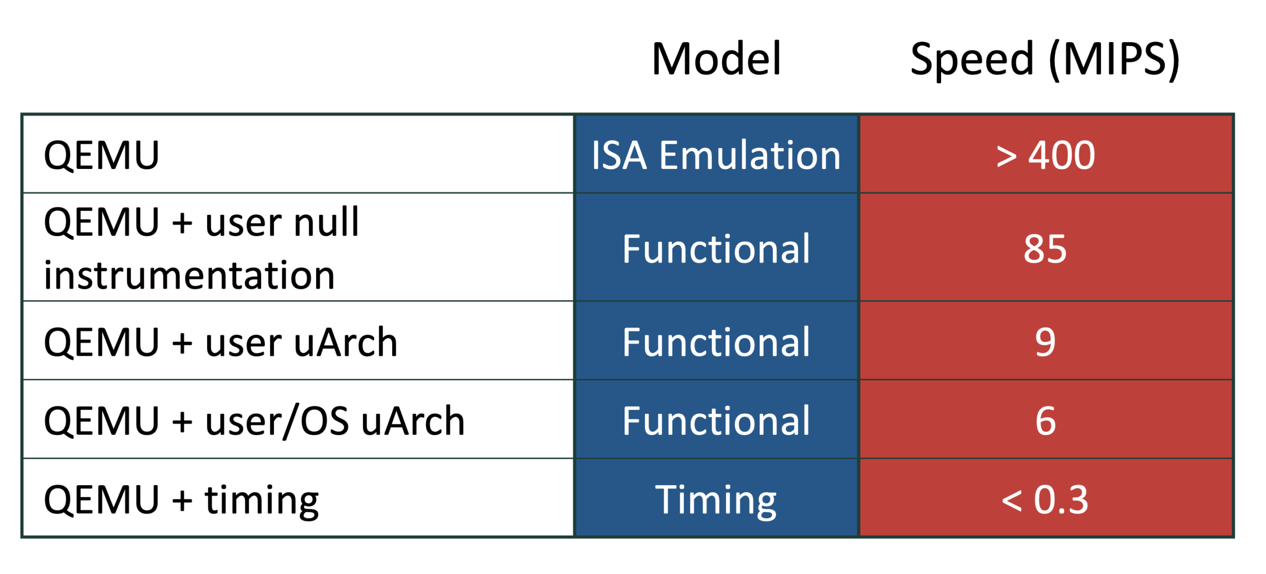

Modern workloads are not steady streams of similar instructions. Their performance fluctuates over time due to network activity, resource contention, background OS activity, synchronization effects, software hiccups, DVFS throttling, UI and graphics activity, and other asynchronous events. Alameldeen et al. presented a statistically rigorous methodology to determine the minimum measurement window needed to capture workload performance variability within a specified error bound and confidence level. 

Unlike conventional database workloads (e.g., TPC benchmarks) which have prescribed measurement windows, typical benchmarks and workloads used in research do not. Applying Alameldeen’s methodology, we find that capturing performance variability for a single ARM Neoverse N1 core and its cache hierarchy requires five to 120 seconds of target execution time across server workloads from CloudSuite, DCPerf, and DeathStarBench. Simulating even a few seconds of a single core with today’s fastest cycle-accurate simulator, gem5, at 250 KIPS requires months of simulation time.

What Should We Measure?

The second question is which performance metric to use. Timing simulators count cycles, so architects often report IPC, or instructions per cycle. IPC is reasonable for single-core workloads when most executed instructions correspond to program progress.

For multicore workloads, however, IPC can be misleading. Threads may spin, poll, block, wait on locks, synchronize, or execute OS code that does not advance useful work. A system can therefore sustain high IPC while making little forward progress; in effect, total IPC can reward busy waiting. 

This is why user-level IPC, or U-IPC, is often a better proxy. U-IPC counts user-level instructions over time, assuming that user instructions per request remain roughly stable and that most spinning occurs in the OS. Under that assumption, U-IPC tracks useful throughput more directly than total IPC.

But U-IPC must be validated for each workload. If spinning occurs in user space, as in systems with user-level network stacks, raw U-IPC still counts non-productive work and must be corrected to exclude spinning. The broader requirement is therefore metric validation: a rigorous simulation methodology must show that the chosen metric—IPC, U-IPC, throughput, or latency—actually captures forward progress for the workload under study.

How Should We Measure?

Due to the timing simulation wall, researchers often use abbreviated measurements. The most common technique is to measure a single unit of 100 million to one billion instructions. Unfortunately, depending on where in the execution the fixed measurement is taken from, this technique may lead to inconclusive results or worse, incorrect conclusions. 

Instead, designers often use sampling to capture variability in performance estimates. Phase-based sampling, such as SimPoint, is a popular technique that uses clustering of basic-block vectors (BBVs) to select representative application “phases.” Such sampling properly captures the representing repetitive instruction streams that account for most of the execution. 

While simple and practical, phase-based sampling may ignore OS effects, interrupts and I/O interactions, communication among cores, and software hiccups. Moreover, Wunderlich argues in his thesis that phase-based sampling: (1) misses the microarchitectural footprint of less common instruction streams and their impact on performance, and (2) forgoes any error bounds with confidence in estimates.

A rigorous sampling technique is statistical sampling, such as SMARTS, taking a large sample (e.g., hundreds) of small (e.g., 200k cycles), uniformly distanced measurement units that is representative of execution, not phases in the workload. This technique enables bounding the error in estimates and delivers quantifiable confidence. It also opens an entire plethora of statistical sampling tools to trade off confidence in estimates for measurement in speed and quantify sample divergence to detect bias in estimates.

The figure below compares error magnitude in performance estimates among three abbreviated measurement techniques from full-timing simulation runs of tens of target seconds on a two-core socket with 2.0 GHz ARM Neoverse N1 cores running single-tier, multi-tier and consolidated server workloads (CloudSuite, DCPerf and DeathStarBench). The figure compares the error against the full-timing baselines for: (1) single units of one billion instructions per core starting from three equally distanced positions in the minimum measurement window (i.e., beginning, 1/3 and 2/3 into the population), (2) units of 100 target microseconds (i.e., 200k cycles for a 2.0 GHz clock) including basic-block vectors (BBV) derived from K-means clustering, and (3) a uniform sample (of hundreds) of 100 target microseconds drawn with an error bound of 5% with 95% confidence with statistical sampling. 

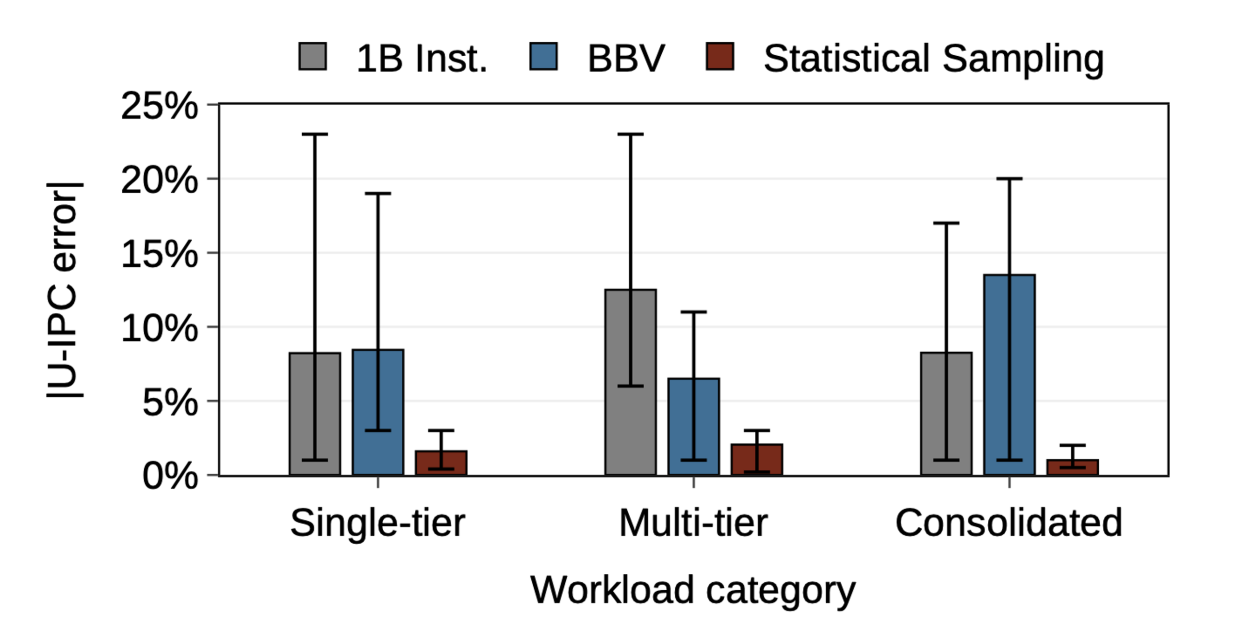
Both one-billion instruction units and BBV result in high error estimates with the former not being representative of execution and the latter representing only frequently executed instructions. In contrast, statistical sampling results in a desired error bound with confidence because it represents not just frequently executed instructions but also instructions that have a high impact on performance due to their microarchitectural footprint.

A SOTA Sampling Framework

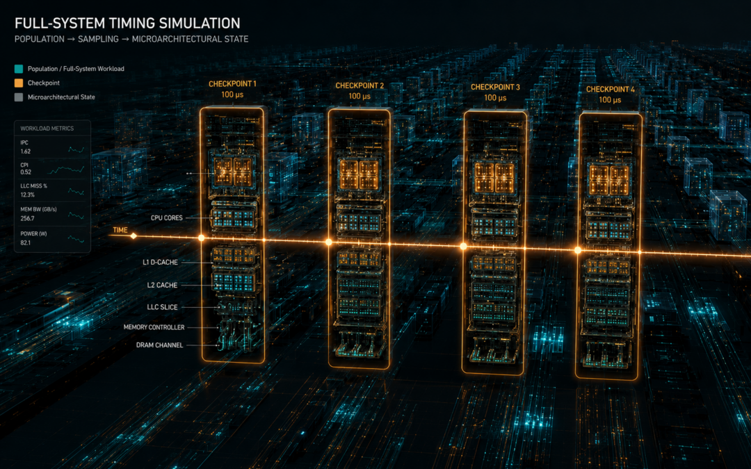
The figure below presents a state-of-the-art sampling framework using QFlex 3.0 (derived from SimFlex) for full-system timing simulation of ARM ISA. For each workload, the software stack together with the OS is first loaded and warmed on a real platform, then tested to identify the minimum window—such as five to 120 target machine’s seconds—called a “population”, using Alameldeen et al.’s technique. The workload is then loaded again, this time with QEMU and run through a functional simulator running on average at 6 MIPS for the entire duration of population. 

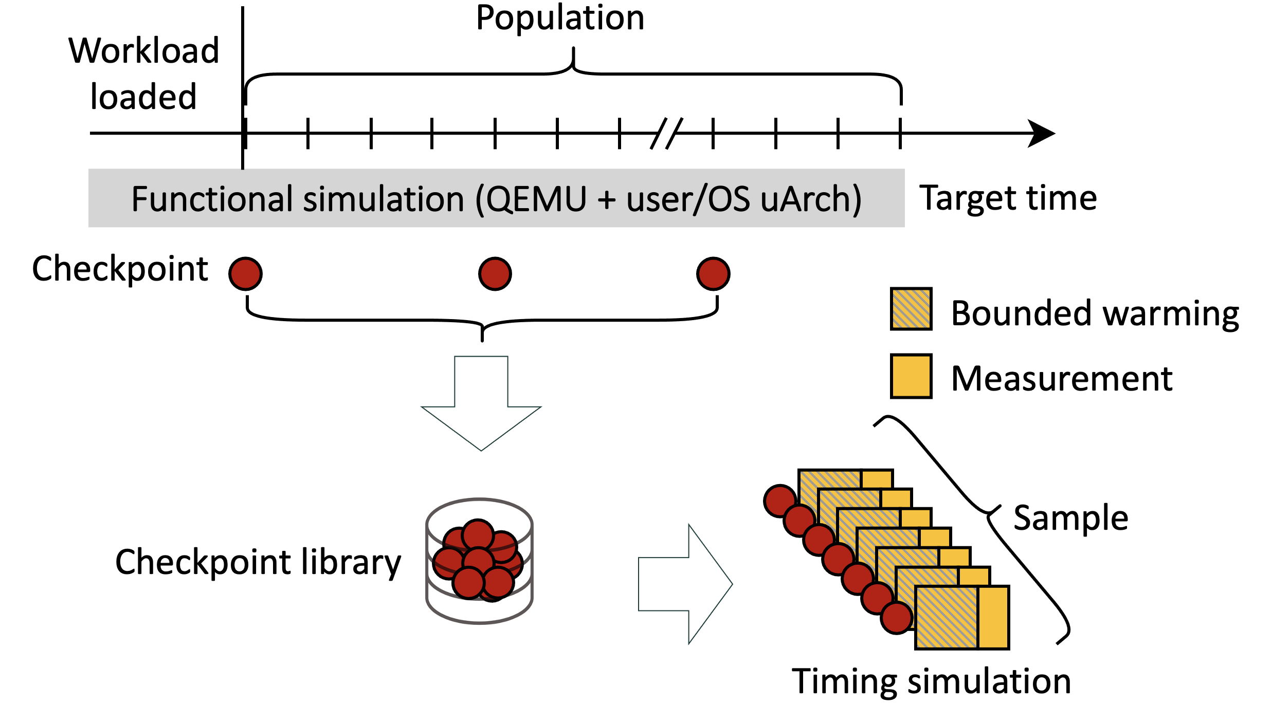
The functional simulator simulates all microarchitectural components with long-term state (e.g., cache hierarchy and TLBs, branch tables, data prefetcher) and periodically dumps checkpoints with architectural and microarchitectural state into a checkpoint library. Because the functional simulator is not cycle-accurate, it requires an approximation for time. The most common approximation is IPC=1 or IPC derived from neighboring units.

The checkpoints in the library are then run using a timing simulator for 100 us independently and embarrassingly parallel. Each checkpoint is first run for a bounded window of time (e.g., 200 us) to make sure microarchitectural components with short-term state (e.g., buffers in the pipeline, cache hierarchy and NoC) are warm, followed by a measurement. The timing results for the sample are then aggregated to determine whether the sample (i.e., number of checkpoints) is large enough to bound the error for a desired level of confidence (e.g., 5% with 95% confidence). If not, the sampling framework creates a new checkpoint library with a shorter interval between checkpoints.

Challenges and Open Problems 

Even with accurate measurement techniques, there are fundamental challenges with sampling (for both phase-based and statistical sampling).

1. Accurate state generation. Timing-induced activity during functional simulation and its impact on the microarchitectural footprint may result in a significant bias because time is approximated. This challenge is more pronounced with variable performance among target threads in multi-tier and consolidated workloads where the speed bias may significantly impact the resulting shared microarchitectural footprint.
2. The functional simulation wall. Sampling minimizes the required measurement using timing simulators but shifts the bottleneck to the functional simulator (which at 6 MIPS is only 24x faster than a 250 KIPs timing simulator). Parallelizing functional simulation may be a promising approach to enable scalability with multicore hosts. Parallel simulation is fundamentally limited by the granularity at which target threads communicate.
3. Support for checkpointing. Generating and restoring an entire checkpoint for every measurement is impractical in both storage capacity and runtime overhead. Practical sampling therefore requires incremental checkpoint storage and restoration.
4. Sampling non-average metrics. Statistical sampling works well for average-like metrics such as IPC or U-IPC, but it is harder to apply to extreme or rare-event metrics such as maximum temperature, worst-case power, or rare latency spikes.
5. Capturing service-level metrics. Metrics such as request latency or p99.9 latency are much coarser-grained than sampling units needed for IPC or U-IPC. Capturing service-level metrics and tail latency may require an order of magnitude larger population and sampling units which poses a challenge for both functional and timing simulation.
6. Multi-node full-system simulation. Many modern workloads are distributed across multiple machines. Single-node simulation is often insufficient for datacenter-scale behavior, but despite progress, rigorous  multi-node full-system timing simulation remains an open challenge.
7. Interoperability across simulators. A practical ecosystem should allow one tool to generate a checkpoint library and another to perform timing simulation. This interoperability requires an interface definition language allowing interoperable architectural and microarchitectural state among simulators.

About the Authors

Shanqing Lin is a final-year PhD student at the School of Computer and Communication Sciences at EPFL and the principal developer of QFlex v3.0.

Mohammad Alian is an Assistant Professor in the Electrical and Computer Engineering Department at Cornell University.

Babak Falsafi is a Professor in the School of Computer and Communication Sciences at EPFL (epfl.ch) and the founding President of Swiss Datacenter Efficiency Association (sdea.ch).

Disclaimer: These posts are written by individual contributors to share their thoughts on the Computer Architecture Today blog for the benefit of the community. Any views or opinions represented in this blog are personal, belong solely to the blog author and do not represent those of ACM SIGARCH or its parent organization, ACM.