Lessons from using an AI coding agent in LLM systems research

This project began with a routing problem. When an LLM request arrives, the system must decide which GPU will execute prefill and which GPU will execute decode. The same GPU can execute both phases. Alternatively, a prefill-only GPU can execute prefill and transfer the request’s key-value, or KV, state to a GPU that executes decode. Local prefill avoids that transfer, but it can lengthen the decode iterations of requests that are already generating tokens on the same GPU. Remote prefill keeps that work off the decoder, but it can add queueing at the prefill-only GPU and delay the request while its KV state is transferred. We wanted a router that considered both the arriving request and the requests already in service.

An AI coding agent made it possible to test this idea quickly. It added instrumentation, generated experiments, replayed the same arrival after forcing different decoder and prefill-path choices, and summarized thousands of measurements. This speed made broad exploration practical. It also allowed a weak experiment to produce a large body of convincing results.

That happened in our project. The agent helped implement the routing rule and produced tidy, reproducible results, but some of those results were scientifically wrong. We later used the same agent to trace metrics through the code and replay the decisions that did not make sense.

The project taught us to give the human, the agent, and the simulator different jobs. We decided what a metric meant, what information the router was allowed to use, and what made a comparison fair. The agent turned those requirements into code and checks. The simulator recorded the queues, batches, and completion times. We used that record to decide whether a result supported our claim.

Local and remote prefill paths

LLM serving has two computational phases. During prefill, a GPU performs the computations over all input tokens and builds the KV state needed to generate output tokens. During decode, a GPU generates the response one token at a time. A GPU that executes both phases is a mixed GPU. We call it local prefill when the selected mixed GPU executes prefill and then decode for the same request. The system can instead execute prefill on a prefill-only GPU and transfer the resulting KV state to a mixed GPU for decode. We call this remote prefill.

Suppose a mixed GPU is already executing decode for twenty requests when a new request with a long input arrives. If that GPU executes the new request’s prefill locally, the request avoids a KV transfer and may receive its first output token sooner. The long prefill, however, extends the GPU iterations shared by the twenty active requests and delays their next tokens. With remote prefill, the new request may wait at the prefill-only GPU and then wait for its KV state to be transferred. During that time, the mixed GPU can continue executing decode for its current batch.

Both choices create delay, but they place it on different requests. We call a request already using an affected resource a resident. A useful router must therefore choose both the decoder and the prefill path while accounting for the residents that share those resources.

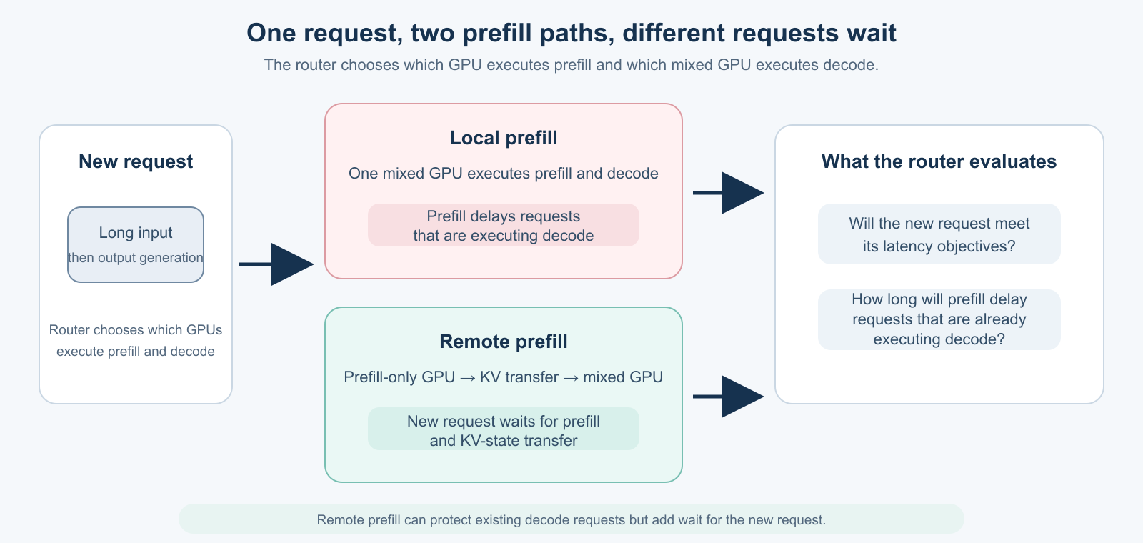
We evaluated each decoder and prefill-path choice using three user-visible delays. These were time to first token, mean time between output tokens, and end-to-end completion time. A request was good only if it met all three latency objectives. Goodput is the fraction of injected requests that were good. The routing idea was simple. The harder problem was to build an experiment that could test it.

The AI coding agent’s implementation role

We built the prototype on BLIS, the Blackbox Inference Simulator. BLIS is an open-source discrete-event simulator created by our team. It advances a simulated clock from one event to the next. An event can be a request arrival or the completion of a GPU iteration. This structure allowed us to replay the same arrivals under different routing choices and inspect the queue, batch, and completion record for each request. The routing extension and experiment harness are separate from the public BLIS repository.

The agent implemented routing rules inside this prototype. It exposed the score assigned to every possible decoder and prefill-path pair, generated workloads, ran the same arrivals under many routing rules, and checked individual request outcomes. We initially expected to supply the research idea while the agent handled implementation and experiments. That division did not hold. Small implementation choices were changing the meaning of the experiment.

The agent could confirm that every run completed. It could also identify which routing rule produced the highest reported goodput. We still had to ask whether that number measured what we intended. Was the event sequence physically possible? Did the router use only information available at decision time? Did every routing rule receive an equally demanding workload? Each of these questions exposed a problem.

Capacity measurement and disaggregation fraction selection

Before comparing routing methods, we had to decide how fast requests should arrive. The same arrival rate can place very different demands on the same fleet. Interactive requests have moderately long inputs and short outputs. Reasoning requests have shorter inputs and much longer outputs. Deep-research requests have very long inputs and short outputs. We therefore needed a separate capacity measurement for each workload. Our simulated fleet contained one prefill-only instance and two mixed instances that could execute both prefill and decode. The disaggregation fraction describes how the prefill work is divided between them. A fraction of 0 keeps every request’s prefill on its selected mixed instance. A fraction of 1 executes every request’s prefill on the prefill-only instance and then transfers its KV state to a mixed instance for decode. On the H100+A100 fleet, we also varied the decoder assignment fraction, which is the fraction of requests whose decode executes on the A100 mixed instance.

Our first attempt used synthetic request streams and tested only disaggregation fractions 0 and 1. For each fraction, the agent tried several offered arrival rates, measured in req/s, and selected the highest rate for which the reported completion rate was at least 95 percent of the offered rate. The intended physical meaning was simple. If 100 requests arrive during an observation period and about 95 finish during that period, the fleet is approximately keeping pace with the arrivals. If only 80 finish, roughly twenty requests have been added to the queue. If that pattern continues, the queue will keep growing. The agent applied this check to both disaggregation fractions and used the larger result as the capacity of the workload and fleet.

When I reviewed the experiment, I asked what this capacity represented physically. Changing the disaggregation fraction changes where work waits. With a fraction of 0, prefill and decode compete for time on the two mixed instances. With a fraction of 1, prefill work can accumulate at the prefill-only instance, while every request must still execute decode on a mixed instance. Different fractions can therefore produce different limiting queues and different completion rates. That is physically reasonable. However, we must first measure the sustained completion rate of each fraction correctly. Only then can we define the empirical capacity of the workload and fleet as the largest rate observed among the fractions we tested.

The agent traced the existing calculation and found that it did not measure sustained service. Each simulation injected a finite sequence of requests. The reported completion rate divided the total number of completions by the time from the beginning of the run until the final request finished. This interval included startup, random gaps between arrivals, busy service, and the final period in which no new requests arrived and the remaining queues drained. One result made the problem visible. An offered rate of 3.0 req/s failed the 95 percent check, while 3.5 req/s passed. The increase in completion rate was not itself suspicious because a higher arrival rate can fill GPU batches and improve execution efficiency. The problem was the resulting classification. The calculation claimed that the fleet could not keep pace at 3.0 req/s but could keep pace at 3.5 req/s. The pass-or-fail decision did not match the physical meaning that we had assigned to it.

We replaced that check with a direct measurement of sustained service. For each workload and fleet, we supplied enough requests to keep the limiting resource busy. We held the disaggregation fraction unchanged during each run. On the H100+A100 fleet, we also held the decoder assignment fraction unchanged. We counted completions only during the middle 80 percent of the run so that startup and final draining did not determine the result. Each fraction combination was tested with three independently generated sequences of arrival times and request lengths. We averaged the number of requests completed per second across these three runs. The largest average among the tested fraction combinations became the measured capacity for that workload and fleet. It was an empirical maximum over the fractions we tested, not a theoretical hardware limit or a production measurement. On the homogeneous H100 fleet, the measured capacities were 14.4 req/s for interactive traffic, 0.256 req/s for reasoning, and 0.939 req/s for deep-research traffic.

This correction answered how fast the fleet could complete requests, but it did not tell us which fractions would provide the strongest fixed comparison for goodput. The agent initially reused the fractions that had maximized completion rate. I asked why a fraction that maximizes completed requests per second should also maximize the fraction of requests meeting their latency objectives. Following one long-input request makes the difference concrete. If a mixed instance executes its prefill locally, that prefill shares the GPU with requests already executing decode and delays their next output tokens. If the prefill-only instance executes the same work, those existing decode requests can continue, but the new request may wait at the prefill-only instance and for its KV-state transfer. When the fleet is saturated, the main question is which division of work lets the fleet finish the most requests per second. Below capacity, both choices may finish every request, but they can make different requests wait. The better disaggregation fraction for goodput is the one that allows more requests to meet all three latency objectives, even if it does not increase the maximum completion rate.

The final experiment therefore made the two selections separately. We first measured capacity using sustained completion rate. We then offered each workload 60, 80, and 95 percent of that capacity and tested the fractions again. This time, we selected the disaggregation fraction and decoder assignment fraction that produced the highest goodput on request sequences reserved for making this choice. After selecting the fractions, we evaluated every routing method four times for each workload, fleet, and offered load. Each repetition used a newly generated sequence of arrival times and request lengths. Every routing method received the same four sequences, and none of them had been used to select the fractions. This reduced the chance that one unusually easy or difficult request sequence would determine the comparison.

The distinction materially changed the experiment. For interactive traffic on the homogeneous H100 fleet, a disaggregation fraction of 0.4 produced the highest sustained completion rate. The fractions that produced the highest goodput were 1.0, 0.8, and 0.9 at low, medium, and high load. Across all 18 workload, fleet, and load combinations, choosing fractions for goodput rather than capacity raised their mean goodput from 0.9198 to 0.9296. At 95 percent load for homogeneous interactive traffic, goodput rose from 0.902 to 0.944. These fractions still did not form an oracle. They specified how many requests would execute prefill remotely, but not which individual requests would benefit most. They also could not react to cached tokens, live queues, or requests already executing.

Goodput tuning removed most of the apparent advantage over fixed routing. The resident-aware router nevertheless remained the most robust tested routing method that reacted to the current system state. It performed better than the goodput-tuned fractions in 11 of the 18 combinations, tied in three, and performed worse in four. Its benefit was not a universal or dramatic increase in goodput. It was the ability to remain close to the best result across workloads and loads without knowing the best disaggregation fraction in advance. The agent could run both sets of experiments once we defined them. Human judgment was needed to recognize that sustained completion rate and latency-objective attainment were separate scientific questions. The smaller final advantage was more credible precisely because the comparison had become harder.

Output-length leakage in the deployable estimator

Another problem appeared in an admission-delay estimator. We kept an oracle estimator for diagnosis and deliberately allowed it to use the output length that a request would eventually produce. The deployable estimator could use only information available when the router made its decision. During implementation, both estimators received the same diagnostic record, which contained the realized output length. The deployable estimator used that value.

The contaminated estimator produced a median ratio of realized to predicted admission delay of 1.29. A ratio of 1.0 would be exact, while 1.29 meant that the realized delay was 29 percent larger than the prediction. The result passed our first checks. We then asked why the deployable and oracle outputs were identical when their estimated and realized output lengths were different.

The agent followed the value through the sequence of function calls and found the leak. We separated the data passed to the two estimators, prevented the deployable estimator from using the future output length, and withdrew the 1.29 result. The arithmetic had been tested, but the experiment had not enforced the intended information boundary. We had to define that boundary. The agent then checked every function that could pass future information to the deployable estimator.

Overlapping intervals in the remote-prefill estimator

An early estimate for remote prefill added four intervals. They were prefill queueing and execution, KV-state transfer, the decoder queue seen at arrival time, and the first decode iteration. Each interval was real. The problem was that some of them passed at the same time.

Suppose remote prefill and KV-state transfer take 8 ms while 6 ms of the original decoder queue clears. When the KV state reaches the decoder, only 8 ms has passed. The old estimate reported 14 ms because it added both intervals in full. This double counting made remote prefill look more expensive than it was. Only the part of the decoder wait that remains after the transfer can delay admission.

We asked which event had to finish before the next event could begin and which events could overlap. The agent replayed their timestamps and showed where the intervals overlapped. Our first repair removed the double count. The final estimator advanced the scheduler state one simulated iteration at a time until the request was admitted and produced its first token. More samples could not repair the old formula because we had to correct the order of events.

The human, agent, and simulator workflow

We did not begin with a complete specification for the agent to execute. Results from the implementation often exposed a contradiction. We used the contradiction to state the scientific requirement more clearly and ran the experiment again. The investigation usually followed four steps.

1. We stated the required physical behavior, the information available when the router acted, and the request sequence that every routing rule had to receive.
2. The agent made that requirement observable. It traced a metric to the code that computed it, exposed hidden state, replayed events, or tested values near a pass-or-fail threshold.
3. BLIS produced each request’s history and reran the same arrival while forcing a different decoder or prefill path.
4. We changed the implementation, protocol, or claim to match the measured record. Then we repeated the process.

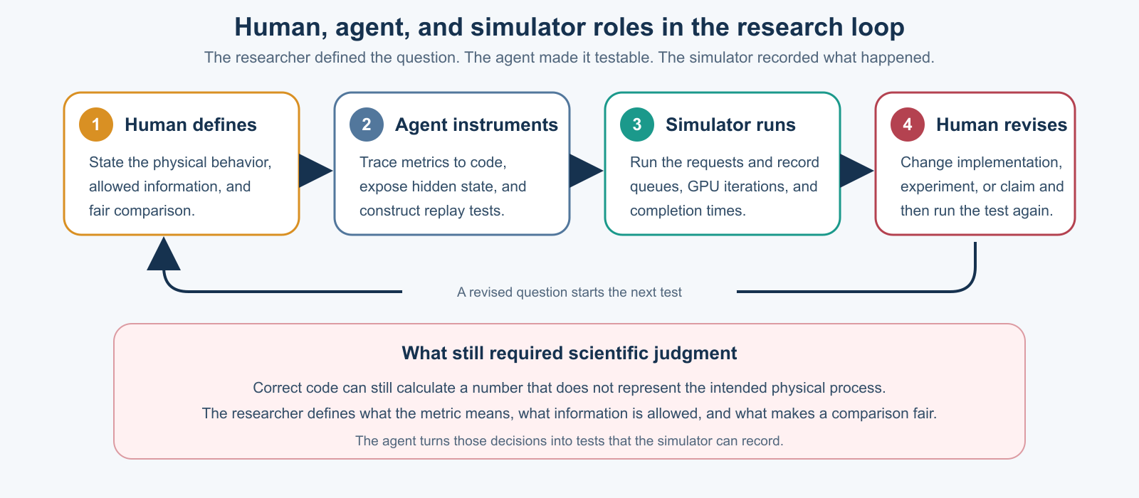
The simulator did not choose the research question, and the agent did not decide what the experiment should mean. Those decisions remained ours. We compared the simulator record with the physical requirements we had stated. The system had the final word on the implemented experiment because its record showed whether the implementation supported the claim.

Strengths and limitations of the AI coding agent

The agent worked best when a result could be checked against a concrete record. It instrumented every possible decoder and prefill-path pair, reran an arrival with local and remote prefill, gave each routing rule the same request arrival times and token counts, verified that each request reached exactly one outcome, and located the code that produced a number. It also reduced the cost of being wrong. We could test an explanation and discard it without treating the implementation effort as a reason to defend it.

It was less reliable when correctness depended on the meaning of the model. The agent could test a calculation without recognizing that the calculation described the wrong physical process. The program could be correct while the scientific claim was not.

The agent usually accepted the quantity or relationship named in the task. If we described queueing delay as a sum, it implemented and tested that sum. If an experiment script labelled an arrival rate as the largest sustainable rate, it analyzed results at that rate. Progress came when we asked what the calculation represented in the physical system. The agent then answered each question with code, event records, and repeatable experiments. This combination let us inspect far more evidence than we could have handled manually.

Corrected benchmark design and results

After these corrections, the final benchmark covered three workloads and two fleets at offered rates equal to 60, 80, and 95 percent of measured capacity. This produced 18 workload, fleet, and offered-rate combinations. We tested three routing rules that chose a decoder and a prefill path for every arriving request while observing the current system state. We also tested two ways of keeping the disaggregation fraction and decoder assignment fraction unchanged during a run. One used the fractions that had produced the highest sustained completion rate. The other used the fractions that had produced the highest goodput on separate request sequences reserved for making that choice. All five routing rules then ran on four new request sequences that had not been used to choose rates or fractions. This produced 360 runs. Every submitted request completed, and none was dropped, timed out, or truncated.

Across the 18 workload, fleet, and offered-rate combinations, the resident-aware router achieved a mean goodput of 0.9327 when every combination received equal weight. For each combination, we averaged each of the three routing rules that observed current system state over the four new request sequences. We then compared the resident-aware router with the largest of those three averages for that same combination. This did not select one routing rule after viewing the full benchmark. The resident-aware router’s largest shortfall was 0.0125, which corresponds to 1.25 fewer good requests per 100 arrivals in that combination. Its mean goodput was 0.0031 higher than the result obtained with goodput-tuned fixed fractions.

The corrected comparison changed the conclusion. The resident-aware router still ranked first among the three routing rules that observed current system state, but its advantage over the goodput-tuned fixed fractions was small. The evidence supported a claim about robustness across the tested conditions, not a universal win.

Methodology for AI-assisted systems research

Our experience suggests a practical role for AI in systems research. For every scientific claim, ask the agent to build a trace, replay, test, or implementation that could prove the claim wrong.

We now ask four questions about every major result. What physical event or resource does the metric represent? What information is available when the system acts? Do the load and controls produce a fair comparison? What can the evidence establish, and what would make us withdraw the claim?

The human researcher remains responsible for these questions because they define the object being studied. The agent can make the answers visible in traces, invariants, matched replays, and repeatable experiments. The system then supplies the record used to judge the claim.

Lessons from the study

The agent made it easy to run experiments, which made the quality of each question more important. A vague question could produce hundreds of completed experiments before we noticed the ambiguity. A precise question could be tested at a depth that had previously been impractical. We learned to use each part of the collaboration for a different purpose. We challenged the meaning of a result, the agent challenged the implementation through traces and replays, and the simulator showed whether the implementation behaved as required.

The routing rule was one outcome of this project, but the broader contribution was an AI-native research method. The agent did not replace scientific judgment. It reduced the cost of turning a question into instrumented code, running controlled comparisons, and tracing a surprising result back to the events that produced it.

The central lesson is to use that speed to make claims easier to challenge, not merely faster to produce. The researcher must define what a metric means physically, what information the system may use, and what makes a comparison fair. The agent can turn those decisions into tests and expose where the implementation violates them. The researcher frames the question, the agent makes it testable, and the system record has the final word.

About the author

Vishakha Ramani is a Research Staff Member at the IBM T. J. Watson Research Center, where she works at the intersection of theory and systems, with a focus on large-scale LLM inference and cloud platforms. She received her M.S. and Ph.D. degrees in Electrical and Computer Engineering from Rutgers University in 2020 and 2024, respectively, and conducted her graduate research at WINLAB. Her research applies performance modeling, queueing theory, and systems experimentation to improve latency, throughput, and information freshness in distributed and AI systems.

 

Disclaimer: These posts are written by individual contributors to share their thoughts on the Computer Architecture Today blog for the benefit of the community. Any views or opinions represented in this blog are personal, belong solely to the blog author and do not represent those of ACM SIGARCH or its parent organization, ACM.